Approach
We study two objectives for multimodal representation learning. The first is cross-alignment (CA),
which aligns paired samples in a shared latent space. The second is cross-prediction (CP),
which predicts one modality from the other through an encoder–decoder factorization. Both are formalized below:
Let \(f_X : \mathbb{R}^{d_x} \to \mathbb{R}^k\) and \(f_Y : \mathbb{R}^{d_y} \to \mathbb{R}^k\) be encoders
producing latent codes \(\mathbf{z}_x^{(i)} := f_X(\mathbf{x}_i)\) and \(\mathbf{z}_y^{(i)} := f_Y(\mathbf{y}_i)\)
in a shared latent space of dimension \(k\). Let \(f_D : \mathbb{R}^k \to \mathbb{R}^{d_y}\) be a decoder.
The two objectives are
\[
\begin{aligned}
\text{(CA)} \quad &\min_{f_X,\, f_Y} \;
\tfrac{1}{n} \textstyle\sum_i \| f_X(\mathbf{x}_i) - f_Y(\mathbf{y}_i) \|_2^2
\quad \text{s.t.} \quad
\tfrac{1}{n} \textstyle\sum_i f_X(\mathbf{x}_i)\, f_Y(\mathbf{y}_i)^\top = \mathbf{I}_k,
\\[6pt]
\text{(CP)} \quad &\min_{f_X,\, f_D} \;
\tfrac{1}{n} \textstyle\sum_i \| \mathbf{y}_i - f_D(f_X(\mathbf{x}_i)) \|_2^2.
\end{aligned}
\]
With linear encoders \(f_X(\mathbf{x}) = W\mathbf{x}\), \(f_Y(\mathbf{y}) = V\mathbf{y}\) for CA, and
linear encoder \(f_X(\mathbf{x}) = E\mathbf{x}\) and decoder \(f_D(\mathbf{z}) = D\mathbf{z}\) for CP,
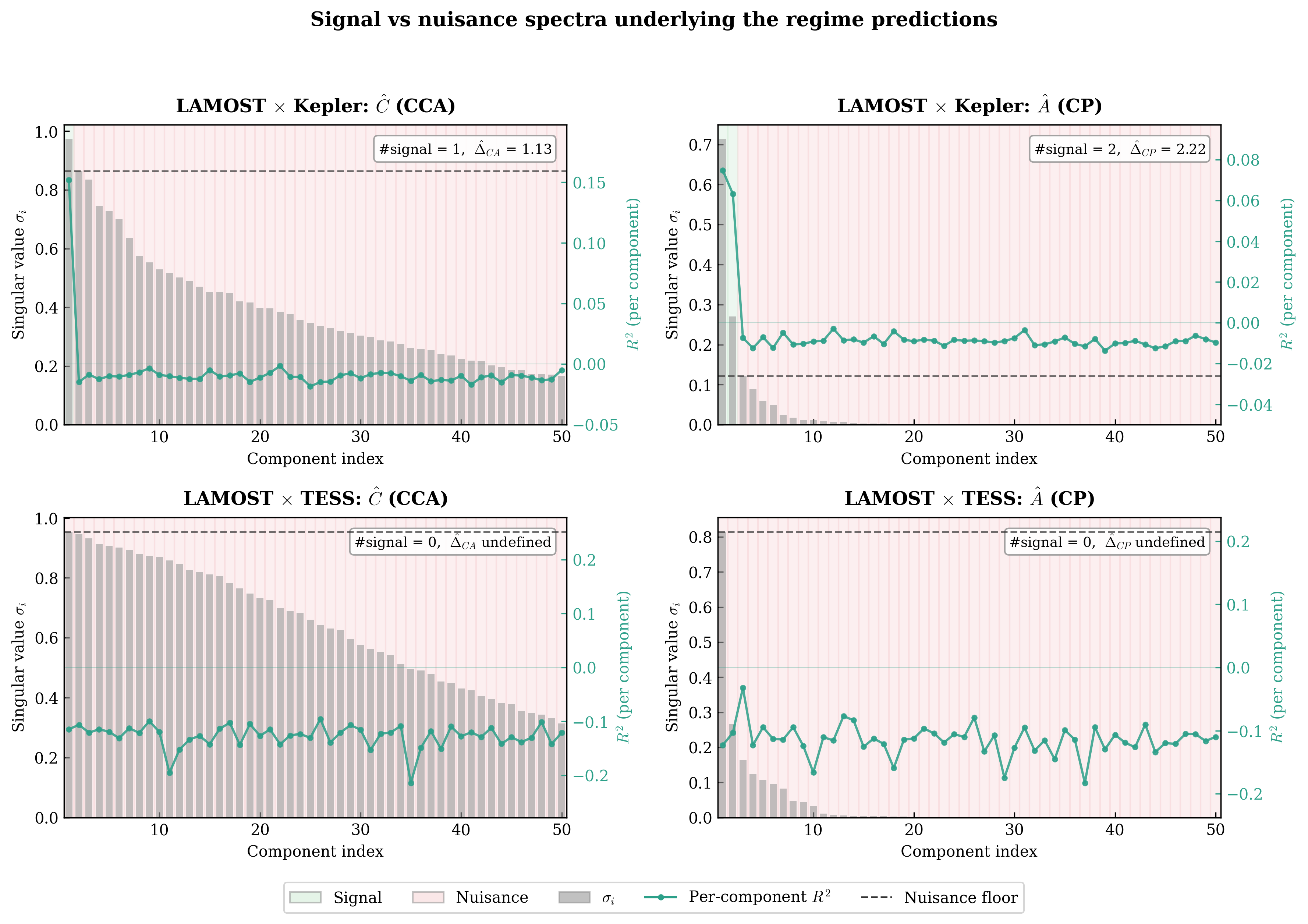
both objectives admit closed-form solutions expressible through the SVDs of two modality-coupling matrices:
\[
C := \Sigma_{xx}^{-1/2}\, \Sigma_{xy}\, \Sigma_{yy}^{-1/2}, \qquad
A := \Sigma_{yx}\, \Sigma_{xx}^{-1/2},
\]
where \(\Sigma_{xx}, \Sigma_{yy}, \Sigma_{xy}\) denote the (population) (cross-)covariances.
To analyze recovery, we posit a signal-plus-noise model in which each modality decomposes into \(k\) shared
signal coordinates and \(d - k\) modality-specific nuisance coordinates.
The singular values of \(C\) and \(A\) split into signal values \(\{\rho_i,\,\tau_i\}_{i=1}^{k}\) and nuisance
values \(\{\nu_j,\,\xi_j\}_{j=1}^{d-k}\), given by
\[
\rho_i = \frac{\kappa_i^2}{\sqrt{(\kappa_i^2 + \gamma_i^x)(\kappa_i^2 + \gamma_i^y)}},
\quad
\tau_i = \frac{\kappa_i^2}{\sqrt{\kappa_i^2 + \gamma_i^x}},
\quad
\nu_j = \frac{\eta_j}{\sqrt{\tilde{\gamma}_j^x\, \tilde{\gamma}_j^y}},
\quad
\xi_j = \frac{\eta_j}{\sqrt{\tilde{\gamma}_j^x}}.
\]
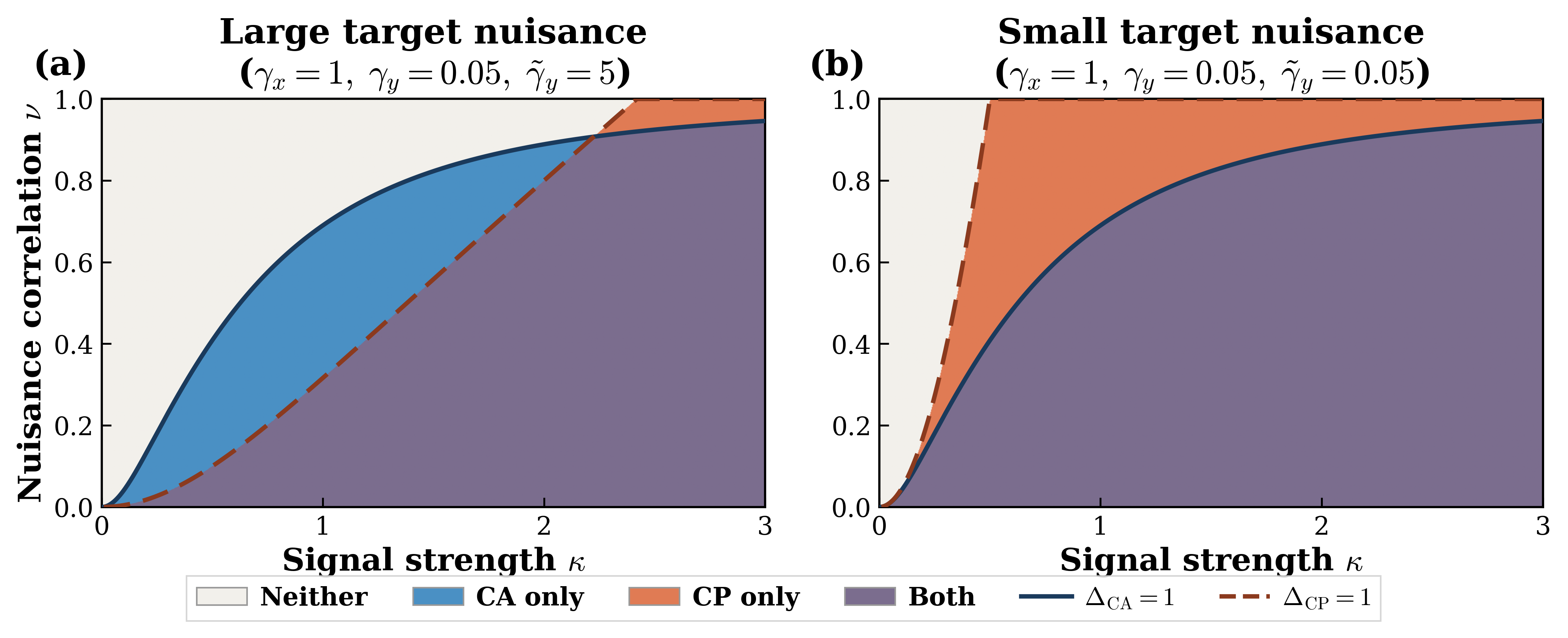
CA (resp. CP) fully recovers the shared signal subspace whenever its signal singular values exceed its nuisance
singular values. Defining the ratio of signal to nuisance singular values as the separation ratios, we define
4 different recovery regimes — Both, CP only, CA only, and Neither — as described in the following table:
| Region |
CA recovers? |
CP recovers? |
| Both | ✓ | ✓ |
| CA only | ✓ | ✗ |
| CP only | ✗ | ✓ |
| Neither | ✗ | ✗ |
Each method shine and fall under different scenarios: CA is symmetric and preferable when modality-specific noise is large or uncertain. CP is assymetric, requires the correct source-target direction, and is preferable when signal is strong and the modality-specific noise is weak.
Importatnly, the Neither regime is a carachteristic of real world problems with complementary modaitlies, and low signal-to-noise ratio. This regime requires novel alignment methods, beyond simple CA or CP.